    Welch Two Sample t-test

data:  LogRT by Affix
t = 2.5034, df = 421.23, p-value = 0.01268
alternative hypothesis: true difference in means between group bar and group ede is not equal to 0
95 percent confidence interval:
 0.01095439 0.09103241
sample estimates:
mean in group bar mean in group ede
6.795550 6.744556 Repetir o script não garante reproduzir a análise:
as decisões do pesquisador como grau de liberdade
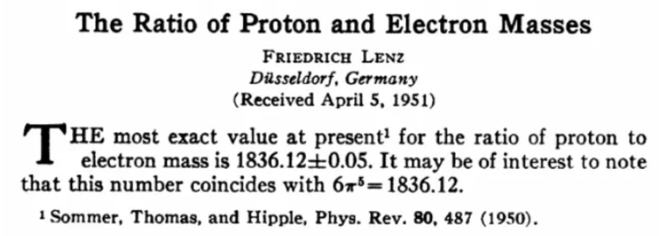
LENZ, Friedrich. The ratio of proton and electron masses. Physical Review, v. 82, n. 4, p. 554, 1951.
Exemplo 2 (McElreath 2020)
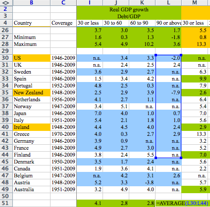
- 2010: “Growth in a time of debt” by Reinhart & Rogoff
- 2013: “Does High Public Debt Consistently Stifle Economic Growth? A Critique of Reinhart and Rogoff” by Herndon, Ash & Pollin


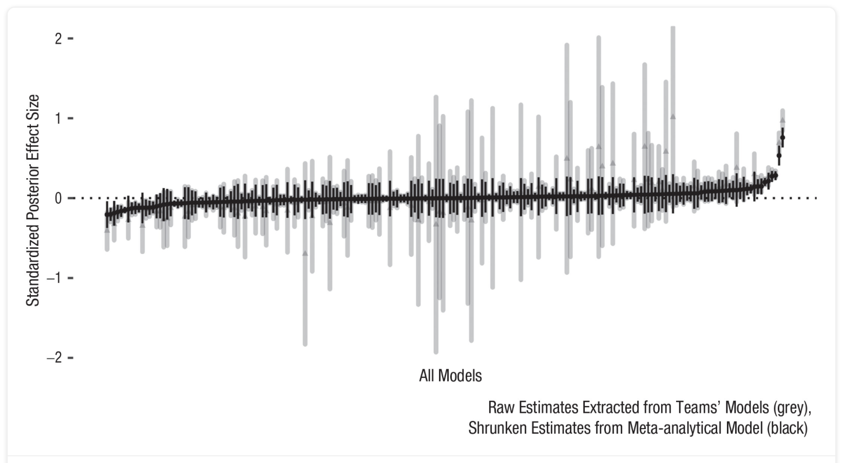
“In light of this idiosyncratic variability, we recommend that researchers more transparently share details of their analysis, strengthen the link between theoretical construct and quantitative system, and calibrate their (un)certainty in their conclusions.”
Exemplo 1:
Lima Jr & Garica (2021)
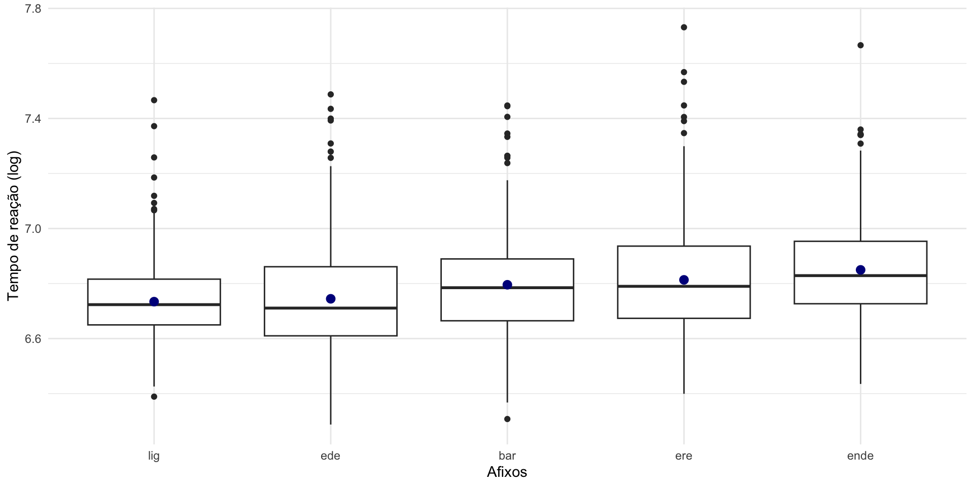
- Pergunta de pesquisa: tem diferença entre “ede” e “bar”?
Exemplo 3
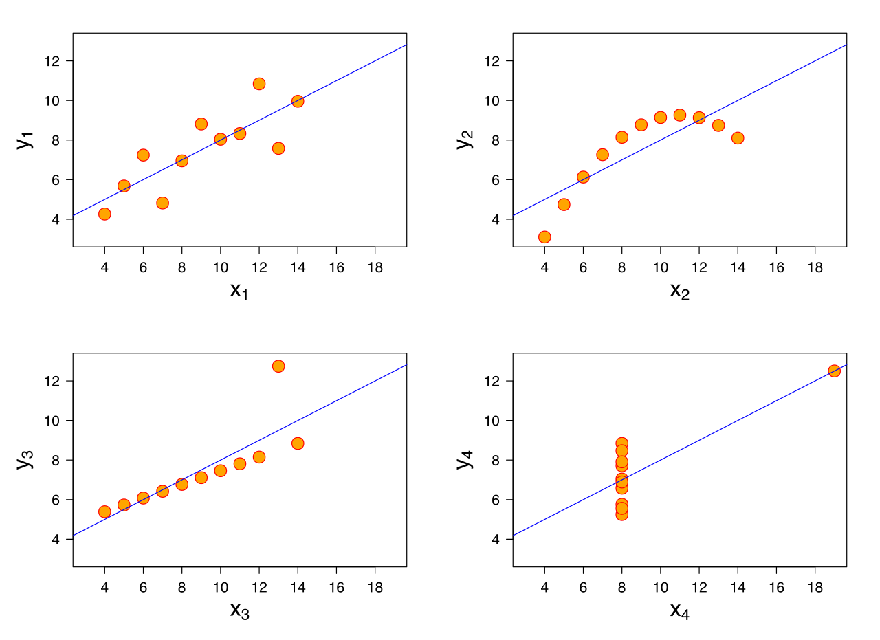
O quarteto de Anscombe (1973)
- \(\bar{X}\) de x = 9
- \(s\) de x = 3,3
- \(\bar{X}\) de y = 7,5
- \(s\) de y = 2
- Corr de x e y = 0,816
- Regressão linear: \(y = 3+0,5x\)
- \(R^2=0,67\)
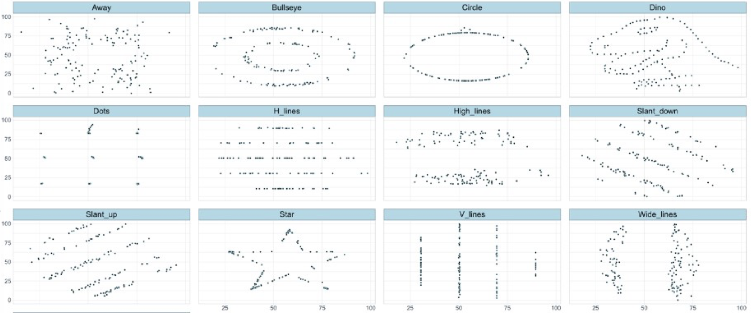
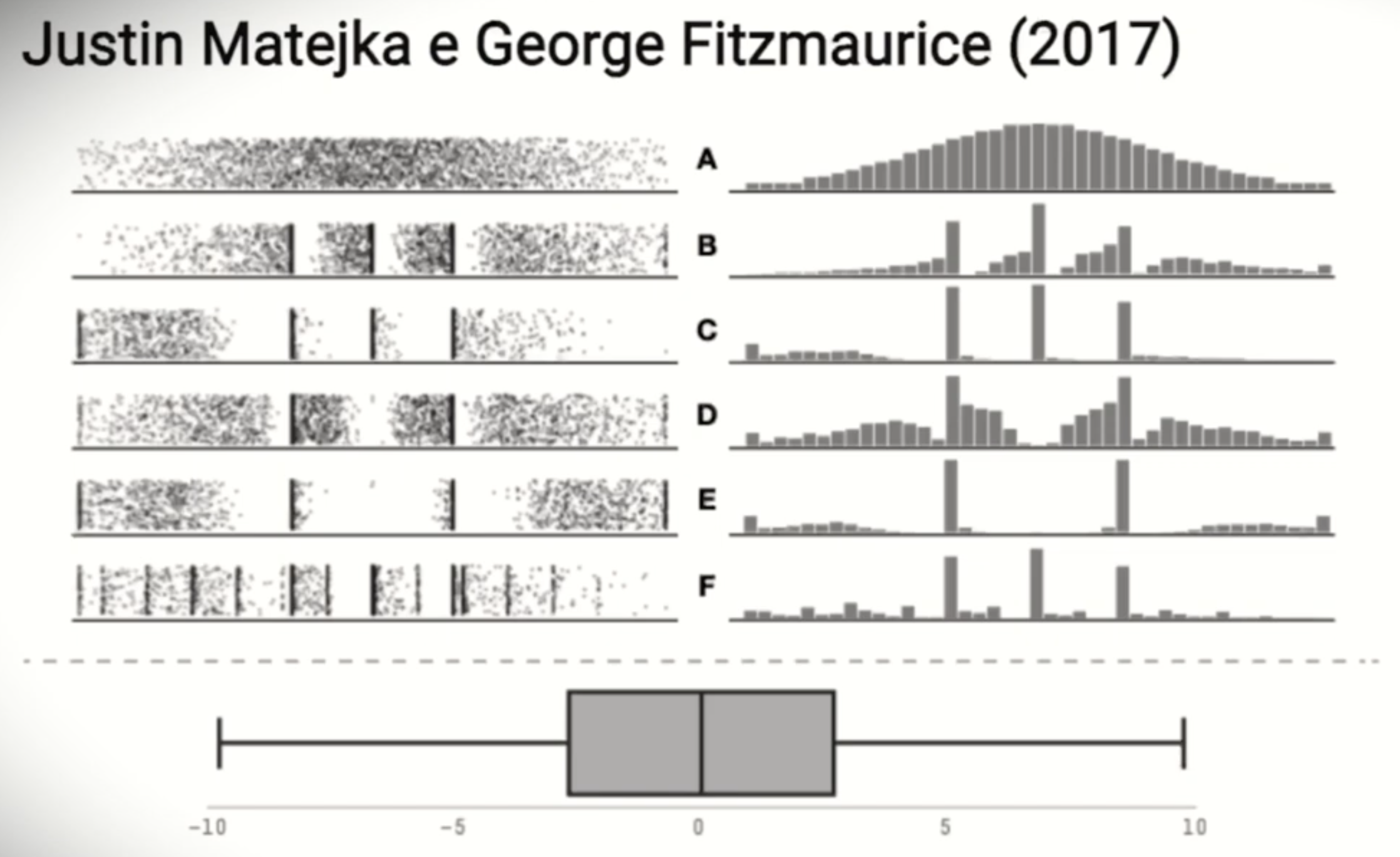
Datasaurus dozen
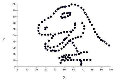
Datasaurus dozen
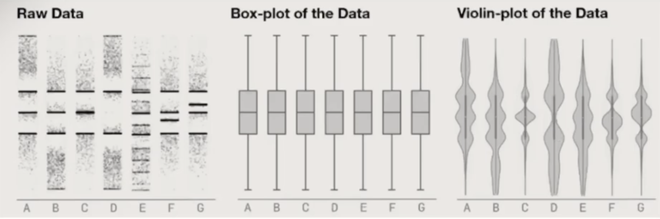
Boxplot
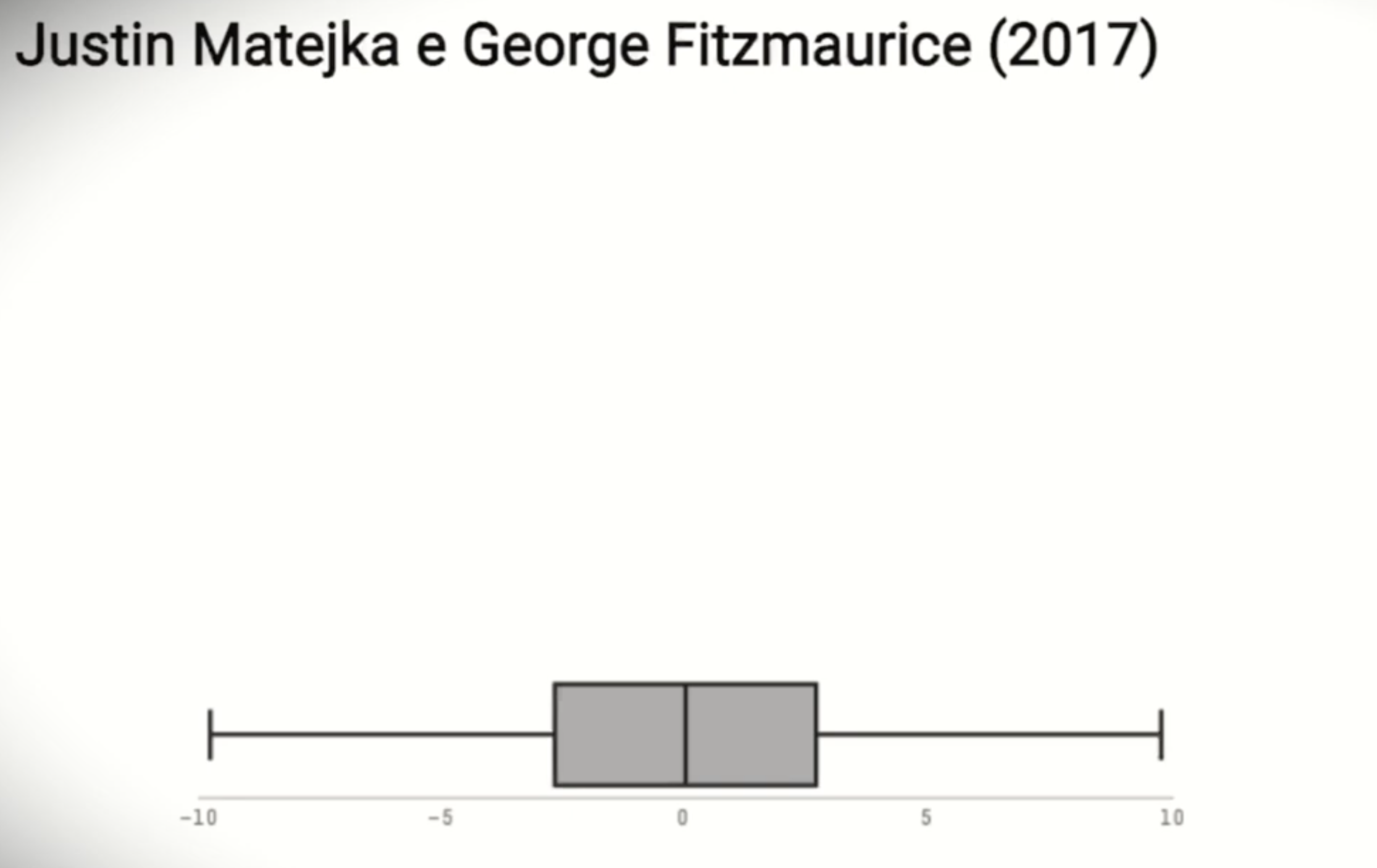
Boxplot
Boxplot
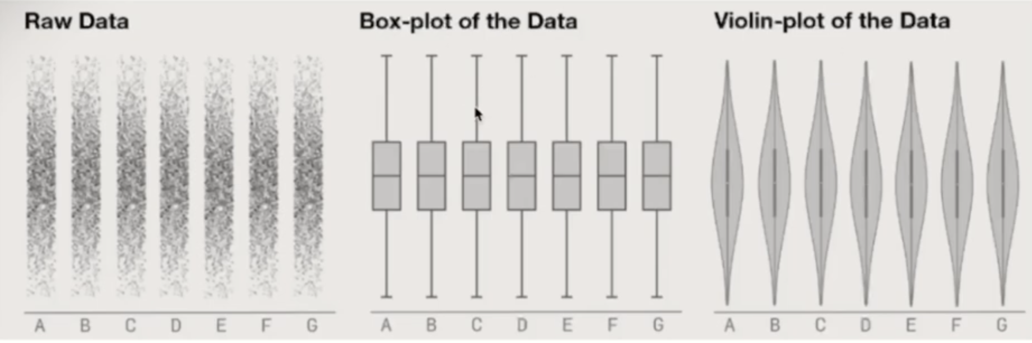
Boxplot
Slides:
@ronaldolimajunior